This notebook explans how to use the pandas library for analysis of tabular data.
# Start using pandas (default import convention)
import pandas as pd
import numpy as np
# Let pandas speak for themselves
print(pd.__doc__)
pandas - a powerful data analysis and manipulation library for Python
=====================================================================

**pandas** is a Python package providing fast, flexible, and expressive data
structures designed to make working with "relational" or "labeled" data both
easy and intuitive. It aims to be the fundamental high-level building block for
doing practical, **real world** data analysis in Python. Additionally, it has
the broader goal of becoming **the most powerful and flexible open source data
analysis / manipulation tool available in any language**. It is already well on
its way toward this goal.

Main Features
-------------
Here are just a few of the things that pandas does well:

  - Easy handling of missing data in floating point as well as non-floating
    point data.
  - Size mutability: columns can be inserted and deleted from DataFrame and
    higher dimensional objects
  - Automatic and explicit data alignment: objects can be explicitly aligned
    to a set of labels, or the user can simply ignore the labels and let
    `Series`, `DataFrame`, etc. automatically align the data for you in
    computations.
  - Powerful, flexible group by functionality to perform split-apply-combine
    operations on data sets, for both aggregating and transforming data.
  - Make it easy to convert ragged, differently-indexed data in other Python
    and NumPy data structures into DataFrame objects.
  - Intelligent label-based slicing, fancy indexing, and subsetting of large
    data sets.
  - Intuitive merging and joining data sets.
  - Flexible reshaping and pivoting of data sets.
  - Hierarchical labeling of axes (possible to have multiple labels per tick).
  - Robust IO tools for loading data from flat files (CSV and delimited),
    Excel files, databases, and saving/loading data from the ultrafast HDF5
    format.
  - Time series-specific functionality: date range generation and frequency
    conversion, moving window statistics, date shifting and lagging.
Visit the official website for a nicely written documentation: https://
# Current version (should be 1.5+ in 2023)
print(pd.__version__)
2.2.3
Basic objects
The pandas library has a vast API with many useful functions. However, most of this revolves around two important classes:
Series
DataFrame
In this introduction, we will focus on them - what each of them does and how they relate to each other and numpy objects.
Series
Series is a one-dimensional data structure, central to pandas.
For a complete API, visit https://
# My first series
series = pd.Series([11, 12, 13])
series
0 11
1 12
2 13
dtype: int64This looks a bit like a Numpy array, does it not?
Actually, in most cases the Series wraps a Numpy array...
series.values # The result is a Numpy arrayarray([11, 12, 13])But there is something more. Alongside the values, we see that each item (or “row”) has a certain label. The collection of labels is called index.
series.indexRangeIndex(start=0, stop=3, step=1)This index (see below) can be used, as its name suggests, to index items of the series.
# Return an element from the series
series.loc[1]np.int64(12)# Or
series[1]np.int64(12)# Construction from a dictionary
series_ab = pd.Series({"a": 2, "b": 4})
series_aba 2
b 4
dtype: int64series_ab.loc["a"]np.int64(2)Exercise: Create a series with 5 elements.
result = ...DataFrame
A DataFrame is pandas’ answer to Excel sheets - it is a collection of named columns (or, in our case, a collection of Series). Quite often, we directly read data frames from an external source, but it is possible to create them from:
a dict of Series, numpy arrays or other array-like objects
from an iterable of rows (where rows are Series, lists, dictionaries, ...)
# List of lists (no column names)
table = [
    ['a', 1],
    ['b', 3],
    ['c', 5]
]
table_df = pd.DataFrame(table)
table_df# Dict of Series (with column names)
df = pd.DataFrame({
'number': pd.Series([1, 2, 3, 4], dtype=np.int8),
'letter': pd.Series(['a', 'b', 'c', 'd'])
})
df# Numpy array (10x2), specify column names
data = np.random.normal(0, 1, (10, 2))
df = pd.DataFrame(data, columns=['a', 'b'])
df# A DataFrame also has an index.
df.indexRangeIndex(start=0, stop=10, step=1)# ...that is shared by all columns
df.index is df["a"].indexTrue# The columns also form an index.
df.columnsIndex(['a', 'b'], dtype='object')Exercise: Create DataFrame whose x-column is , y column is cos(x) and index are fractions 0, 1/4, 1/2 ... 2
import fractions

index = [fractions.Fraction(n, ___) for n in range(___)]
x = np.___([___ for ___ in ___])
y = ___

df = pd.DataFrame(___, index = ___)

# display
df
---------------------------------------------------------------------------
TypeError Traceback (most recent call last)
Cell In[18], line 3
1 import fractions
----> 3 index = [fractions.Fraction(n, ___) for n in range(___)]
4 x = np.___([___ for ___ in ___])
5 y = ___
TypeError: 'RangeIndex' object cannot be interpreted as an integerD(ata) types
Pandas builds upon the numpy data types (mentioned earlier) and adds a couple of more.
typed_df = pd.DataFrame({
  "bool": np.arange(5) % 2 == 0,
  "int": range(5),
  "int[nan]": pd.Series([np.nan, 0, 1, 2, 3], dtype="Int64"),
  "float": np.arange(5) * 3.14,
  "complex": np.array([1 + 2j, 2 + 3j, 3 + 4j, 4 + 5j, 5 + 6j]),
  "object": [None, 1, "2", [3, 4], 5 + 6j],
  "string?": ["a", "b", "c", "d", "e"],
  "string!": pd.Series(["a", "b", "c", "d", "e"], dtype="string"),
  "datetime": pd.date_range('2018-01-01', periods=5, freq='3M'),
  "timedelta": pd.timedelta_range(0, freq="1s", periods=5),
  "category": pd.Series(["animal", "plant", "animal", "animal", "plant"], dtype="category"),
  "period": pd.period_range('2018-01-01', periods=5, freq='M'),
})
typed_df
/var/folders/dm/gbbql3p121z0tr22r2z98vy00000gn/T/ipykernel_95281/1417085050.py:10: FutureWarning: 'M' is deprecated and will be removed in a future version, please use 'ME' instead.
"datetime": pd.date_range('2018-01-01', periods=5, freq='3M'),
typed_df.dtypesbool bool
int int64
int[nan] Int64
float float64
complex complex128
object object
string? object
string! string[python]
datetime datetime64[ns]
timedelta timedelta64[ns]
category category
period period[M]
dtype: objectWe will see some of the types practically used in further analysis.
Indices & indexing
abc_series = pd.Series(range(3), index=["a", "b", "c"])
abc_series
a 0
b 1
c 2
dtype: int64abc_series.indexIndex(['a', 'b', 'c'], dtype='object')abc_series.index = ["c", "d", "e"] # Changes the labels in-place!
abc_series.index.name = "letter"
abc_seriesletter
c 0
d 1
e 2
dtype: int64table = [
['a', 1],
['b', 3],
['c', 5]
]
table_df = pd.DataFrame(
table,
index=["first", "second", "third"],
columns=["alpha", "beta"]
)
table_dfalpha = table_df["alpha"] # Simple [] indexing in DataFrame returns Series
alphafirst a
second b
third c
Name: alpha, dtype: objectalpha.loc["second"] # Simple [] indexing in Series returns scalar values.'b'A slice with a ["list", "of", "columns"] yields a DataFrame with those columns.
For example:
table_df[["beta", "alpha"]][["column_name"]] returs a DataFrame as well, not Series:
table_df[["alpha"]]There are two ways how to properly index rows & cells in the DataFrame:
locfor label-based indexingilocfor order-based indexing (it does not use the index at all)
Note the square brackets. The mentioned attributes actually are not methods but special “indexer” objects. They accept one or two arguments specifying the position along one or both axes.
loc
first = table_df.loc["first"]
first
alpha a
beta 1
Name: first, dtype: objecttable_df.loc["first", "beta"]np.int64(1)table_df.loc["first":"second", "beta"] # Use ranges (inclusive)first 1
second 3
Name: beta, dtype: int64iloc
table_df.iloc[1]alpha b
beta 3
Name: second, dtype: objecttable_df.iloc[0:4:2] # Select every second rowtable_df.at["first", "beta"]np.int64(1)type(table_df.at)pandas.core.indexing._AtIndexerModifying DataFrames
Adding a new column is like adding a key/value pair to a dict. Note that this operation, unlike most others, does modify the DataFrame.
table_dffrom datetime import datetime
table_df["now"] = datetime.now()
table_dfNon-destructive version that returns a new DataFrame, uses the assign method:
table_df.assign(delta = [True, False, True]).drop(columns=["now"])# However, the original DataFrame is not changed
table_dfDeleting a column is very easy too.
del table_df["now"]
table_dfThe drop method works with both rows and columns (creating a new data frame), returning a new object.
table_df.drop("beta", axis=1)table_df.drop("second", axis=0)Exercise: Use a combination of reset_index, drop and set_index to transform table_df into pd.DataFrame({'index': table_df.index}, index=table_df["alpha"])
results = table_df.___.___.___

# display
result
Let’s get some real data!
I/O in pandas
Pandas can read (and write to) a huge variety of file formats. More details can be found in the official documentation: http://
Most of the functions for reading data are named pandas.read_XXX, where XXX is the format used. We will look at three commonly used ones.
# List functions for input in pandas.

print("\n".join(method for method in dir(pd) if method.startswith("read_")))
read_clipboard
read_csv
read_excel
read_feather
read_fwf
read_gbq
read_hdf
read_html
read_json
read_orc
read_parquet
read_pickle
read_sas
read_spss
read_sql
read_sql_query
read_sql_table
read_stata
read_table
read_xml
Read CSV
Nowadays, a lot of data comes in the textual Comma-separated values format (CSV). Although not properly standardized, it is the de-facto standard for files that are not huge and are meant to be read by human eyes too.
Let’s read the population of U.S. states that we will need later:
territories = pd.read_csv("data/us_state_population.csv")
territories.head(9)The automatic data type parsing converts columns to appropriate types:
territories.dtypesTerritory object
Population float64
Population 2010 int64
Code object
dtype: objectSometimes the CSV input does not work out of the box. Although pandas automatically understands and reads zipped files,
it usually does not automatically infer the file format and its variations - for details, see the read_csv documentation here:
https://
pd.read_csv('data/iris.tsv.gz')...in this case, the CSV file does not use commas to separate values. Therefore, we need to specify an extra argument:
pd.read_csv("data/iris.tsv.gz", sep='\t')See the difference?
Read Excel
Let’s read the list of U.S. incidents when lasers interfered with airplanes.
pd.read_excel("data/laser_incidents_2019.xlsx")Note: This reads just the first sheet from the file. If you want to extract more sheets, you will need to use the pandas.'ExcelFile class. See the relevant part of the documentation.
Read HTML (Optional)
Pandas is able to scrape data from tables embedded in web pages using the read_html function.
This might or might not bring you good results and probably you will have to tweak your
data frame manually. But it is a good starting point - much better than being forced to parse
the HTML ourselves!
tables = pd.read_html("https://en.wikipedia.org/wiki/List_of_laser_types")
type(tables), len(tables)
(list, 9)tables[1]tables[2]Write CSV
Pandas is able to write to many various formats but the usage is similar.
tables[1].to_csv("gas_lasers.csv", index=False)Data analysis (very basics)
Let’s extend the data of laser incidents to a broader time range and read the data from a summary CSV file:
laser_incidents_raw = pd.read_csv("data/laser_incidents_2015-2020.csv")Let’s see what we have here...
laser_incidents_raw.head()laser_incidents_raw.tail()For an unknown, potentially unevenly distributed dataset, looking at the beginning / end is typically not the best idea. We’d rather sample randomly:
# Show a few examples
laser_incidents_raw.sample(10)laser_incidents_raw.dtypesUnnamed: 0 int64
Incident Date object
Incident Time float64
Flight ID object
Aircraft object
Altitude float64
Airport object
Laser Color object
Injury object
City object
State object
timestamp object
dtype: objectThe topic of data cleaning and pre-processing is very broad. We will limit ourselves to dropping unused columns and converting one to a proper type.
# The first three are not needed
laser_incidents = laser_incidents_raw.drop(columns=laser_incidents_raw.columns[:3])

# We convert the timestamp
laser_incidents = laser_incidents.assign(
    timestamp = pd.to_datetime(laser_incidents["timestamp"])
)
laser_incidentslaser_incidents.dtypesFlight ID object
Aircraft object
Altitude float64
Airport object
Laser Color object
Injury object
City object
State object
timestamp datetime64[ns]
dtype: objectCategorical dtype (Optional)
To analyze Laser Color, we can look at its typical values.
laser_incidents["Laser Color"].describe()count 36461
unique 73
top green
freq 32787
Name: Laser Color, dtype: objectNot too many different values.
laser_incidents["Laser Color"].unique()array(['green', 'purple', 'blue', 'unknown', 'red', 'white',
'green and white', 'white and green', 'green and yellow',
'multiple', 'unknwn', 'green and purple', 'green and red',
'red and green', 'green and blue', 'blue and purple',
'red white and blue', 'blue and green', 'blue or purple',
'blue or green', 'yellow/orange', 'blue/purple', 'unkwn', 'orange',
'multi', 'yellow and white', 'blue and white', 'white or amber',
'red and white', 'yellow', 'amber', 'yellow and green',
'white and blue', 'red, blue, and green', 'purple-blue',
'red and blue', 'magenta', 'phx', 'green or blue', 'red or green',
'green or red', 'green, blue or purple', 'blue and red', 'unkn',
'blue-green', 'multi-colored', nan, 'blue-yellow',
'white or green', 'green and orange', 'white-green-red',
'multicolored', 'green-white', 'blue or white', 'green red blue',
'green or white', 'blue -green', 'green-red', 'green-blue',
'multi-color', 'green-yellow', 'red-white', 'blue-purple',
'white-yellow', 'green-purple', 'lavender', 'orange-red',
'blue-white', 'blue-red', 'yellow-white', 'red-green',
'white-green', 'white-blue', 'white-red'], dtype=object)laser_incidents["Laser Color"].value_counts(normalize=True)Laser Color
green 0.899235
blue 0.046790
red 0.012260
white 0.010395
unkn 0.009051
...
red or green 0.000027
white or green 0.000027
blue-yellow 0.000027
multi-colored 0.000027
white-red 0.000027
Name: proportion, Length: 73, dtype: float64This column is a very good candidate to turn into a pandas-special, Categorical data type. (See https://
laser_incidents["Laser Color"].memory_usage(deep=True) # ~60 bytes per item1969532color_category = laser_incidents["Laser Color"].astype("category")
color_category.sample(10)19194 green
1357 green
8379 green
9911 green
26650 green
22866 green
16266 green
32446 green
23370 green
16057 green
Name: Laser Color, dtype: category
Categories (73, object): ['amber', 'blue', 'blue -green', 'blue and green', ..., 'yellow and green', 'yellow and white', 'yellow-white', 'yellow/orange']color_category.memory_usage(deep=True) # ~1-2 bytes per item43088Exercise: Are there any other columns in the dataset that you would suggest for conversion to categorical?
laser_incidents.describe(include="all")Integer vs. float
Pandas is generally quite good at guessing (inferring) number types.
You may wonder why Altitude is float and not int though.
This is a consequence of not having an integer nan in numpy. There’s been many discussions about this.
laser_incidents["Altitude"]0 8500.0
1 40000.0
2 2500.0
3 3000.0
4 11000.0
...
36458 8000.0
36459 11000.0
36460 2000.0
36461 300.0
36462 1000.0
Name: Altitude, Length: 36463, dtype: float64laser_incidents["Altitude"].astype(int)---------------------------------------------------------------------------
IntCastingNaNError Traceback (most recent call last)
Cell In[82], line 1
----> 1 laser_incidents["Altitude"].astype(int)
File ~/workspace/fjfi/python-fjfi/.venv/lib/python3.12/site-packages/pandas/core/generic.py:6643, in NDFrame.astype(self, dtype, copy, errors)
6637 results = [
6638 ser.astype(dtype, copy=copy, errors=errors) for _, ser in self.items()
6639 ]
6641 else:
6642 # else, only a single dtype is given
-> 6643 new_data = self._mgr.astype(dtype=dtype, copy=copy, errors=errors)
6644 res = self._constructor_from_mgr(new_data, axes=new_data.axes)
6645 return res.__finalize__(self, method="astype")
File ~/workspace/fjfi/python-fjfi/.venv/lib/python3.12/site-packages/pandas/core/internals/managers.py:430, in BaseBlockManager.astype(self, dtype, copy, errors)
427 elif using_copy_on_write():
428 copy = False
--> 430 return self.apply(
431 "astype",
432 dtype=dtype,
433 copy=copy,
434 errors=errors,
435 using_cow=using_copy_on_write(),
436 )
File ~/workspace/fjfi/python-fjfi/.venv/lib/python3.12/site-packages/pandas/core/internals/managers.py:363, in BaseBlockManager.apply(self, f, align_keys, **kwargs)
361 applied = b.apply(f, **kwargs)
362 else:
--> 363 applied = getattr(b, f)(**kwargs)
364 result_blocks = extend_blocks(applied, result_blocks)
366 out = type(self).from_blocks(result_blocks, self.axes)
File ~/workspace/fjfi/python-fjfi/.venv/lib/python3.12/site-packages/pandas/core/internals/blocks.py:758, in Block.astype(self, dtype, copy, errors, using_cow, squeeze)
755 raise ValueError("Can not squeeze with more than one column.")
756 values = values[0, :] # type: ignore[call-overload]
--> 758 new_values = astype_array_safe(values, dtype, copy=copy, errors=errors)
760 new_values = maybe_coerce_values(new_values)
762 refs = None
File ~/workspace/fjfi/python-fjfi/.venv/lib/python3.12/site-packages/pandas/core/dtypes/astype.py:237, in astype_array_safe(values, dtype, copy, errors)
234 dtype = dtype.numpy_dtype
236 try:
--> 237 new_values = astype_array(values, dtype, copy=copy)
238 except (ValueError, TypeError):
239 # e.g. _astype_nansafe can fail on object-dtype of strings
240 # trying to convert to float
241 if errors == "ignore":
File ~/workspace/fjfi/python-fjfi/.venv/lib/python3.12/site-packages/pandas/core/dtypes/astype.py:182, in astype_array(values, dtype, copy)
179 values = values.astype(dtype, copy=copy)
181 else:
--> 182 values = _astype_nansafe(values, dtype, copy=copy)
184 # in pandas we don't store numpy str dtypes, so convert to object
185 if isinstance(dtype, np.dtype) and issubclass(values.dtype.type, str):
File ~/workspace/fjfi/python-fjfi/.venv/lib/python3.12/site-packages/pandas/core/dtypes/astype.py:101, in _astype_nansafe(arr, dtype, copy, skipna)
96 return lib.ensure_string_array(
97 arr, skipna=skipna, convert_na_value=False
98 ).reshape(shape)
100 elif np.issubdtype(arr.dtype, np.floating) and dtype.kind in "iu":
--> 101 return _astype_float_to_int_nansafe(arr, dtype, copy)
103 elif arr.dtype == object:
104 # if we have a datetime/timedelta array of objects
105 # then coerce to datetime64[ns] and use DatetimeArray.astype
107 if lib.is_np_dtype(dtype, "M"):
File ~/workspace/fjfi/python-fjfi/.venv/lib/python3.12/site-packages/pandas/core/dtypes/astype.py:145, in _astype_float_to_int_nansafe(values, dtype, copy)
141 """
142 astype with a check preventing converting NaN to an meaningless integer value.
143 """
144 if not np.isfinite(values).all():
--> 145 raise IntCastingNaNError(
146 "Cannot convert non-finite values (NA or inf) to integer"
147 )
148 if dtype.kind == "u":
149 # GH#45151
150 if not (values >= 0).all():
IntCastingNaNError: Cannot convert non-finite values (NA or inf) to integerQuite recently, Pandas introduced nullable types for working with missing data, for example nullable integer.
laser_incidents["Altitude"].astype("Int64")0 8500
1 40000
2 2500
3 3000
4 11000
...
36458 8000
36459 11000
36460 2000
36461 300
36462 1000
Name: Altitude, Length: 36463, dtype: Int64Filtering
Indexing in pandas Series / DataFrames ([]) support also boolean (masked) arrays. These arrays can be obtained by applying boolean operations on them.
You can also use standard comparison operators like <, <=, ==, >=, >, !=.
It is possible to perform logical operations with boolean series too. You need to use |, &, ^ operators though, not and, or, not keywords.
As an example, find all California incidents:
is_california = laser_incidents.State == "California"
is_california.sample(10)
27390 False
5156 False
27181 False
29581 False
25194 False
19519 False
8354 True
23656 False
9596 True
5121 False
Name: State, dtype: boolNow we can directly apply the boolean mask. (Note: This is no magic. You can construct the mask yourself)
laser_incidents[is_california].sample(10)Or maybe we should include the whole West coast?
# isin takes an array of possible values
west_coast = laser_incidents[laser_incidents.State.isin(["California", "Oregon", "Washington"])]
west_coast.sample(10)Or low-altitude incidents?
laser_incidents[laser_incidents.Altitude < 300]Visualization intermezzo
Without much further ado, let’s create our first plot.
# Most frequent states
laser_incidents["State"].value_counts()[:20]
State
California 7268
Texas 3620
Florida 2702
Arizona 1910
Colorado 988
Washington 982
Kentucky 952
Illinois 946
New York 921
Puerto Rico 912
Oregon 895
Tennessee 888
Nevada 837
Pennsylvania 826
Indiana 812
Utah 789
Ohio 750
Georgia 714
North Carolina 605
Missouri 547
Name: count, dtype: int64laser_incidents["State"].value_counts()[:20].plot(kind="bar");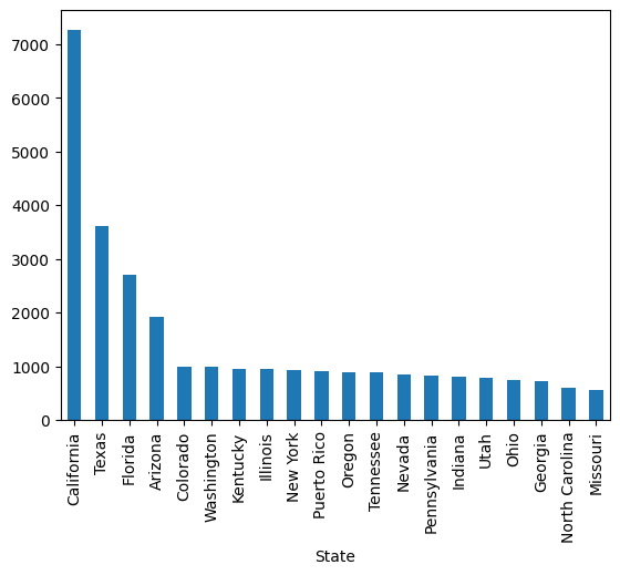
Sorting
# Display 5 incidents with the highest altitude
laser_incidents.sort_values("Altitude", ascending=False).head(5)# Alternative
laser_incidents.nlargest(5, "Altitude")Exercise: Find the last 3 incidents with blue laser.
Arithmetics and string manipulation
Standard arithmetic operators work on numerical columns too. And so do mathematical functions. Note all such operations are performed in a vector-like fashion.
altitude_meters = laser_incidents["Altitude"] * .3048
altitude_meters.sample(10)
23557 2743.20
3239 1310.64
12955 1219.20
2326 1524.00
23309 914.40
6378 1828.80
18797 1828.80
16242 3352.80
1413 5486.40
21954 1066.80
Name: Altitude, dtype: float64You may mix columns and scalars, the string arithmetics also works as expected.
laser_incidents["City"] + ", " + laser_incidents["State"]0 Santa Barbara, California
1 San Antonio, Texas
2 Tampa, Florida
3 Fort Worth , Texas
4 Modesto, California
...
36458 Las Vegas, Nevada
36459 Lincoln, California
36460 Westhampton Beach, New York
36461 Guam, Guam
36462 Naples, Florida
Length: 36463, dtype: objectSummary statistics
The describe method shows summary statistics for all the columns:
laser_incidents.describe()laser_incidents.describe(include="all")laser_incidents["Altitude"].mean()np.float64(7358.314263625822)laser_incidents["Altitude"].std()np.float64(7642.6867120945535)laser_incidents["Altitude"].max()np.float64(240000.0)Basic string operations (Optional)
These are typically accessed using the .str “accessor” of the Series like this:
series.str.lower
series.str.split
series.str.startswith
series.str.contains
...
See more in the documentation.
laser_incidents[laser_incidents["City"].str.contains("City", na=False)]["City"].unique()array(['Panama City', 'Oklahoma City', 'Salt Lake City', 'Bullhead City',
'Garden City', 'Atlantic City', 'Panama City ', 'New York City',
'Jefferson City', 'Kansas City', 'Rapid City', 'Tremont City',
'Boulder City', 'Traverse City', 'Cross City', 'Brigham City',
'Carson City', 'Midland City', 'Johnson City', 'Ponca City',
'Panama City Beach', 'Sioux City', 'Bay City', 'Silver City',
'Pueblo City', 'Iowa City', 'Calvert City', 'Crescent City',
'Oak City', 'Falls City', 'Salt Lake City ', 'Royse City',
'Kansas City ', 'Bossier City', 'Baker City', 'Ellwood City',
'Dodge City', 'Garden City ', 'Union City', 'King City',
'Kansas City ', 'Mason City', 'Plant City ', 'Lanai City',
'Tell City', 'Yuba City', 'Kansas City ', 'Salt Lake City ',
'Kansas City ', 'Ocean City', 'Cedar City', 'City of Commerce',
'Lake City', 'Beach City', 'Alexander City', 'Siler City',
'Charles City', 'Malad City ', 'Rush City', 'Webster City',
'Plant City'], dtype=object)laser_incidents[laser_incidents["City"].str.contains("City", na=False)]["City"].str.strip().unique()array(['Panama City', 'Oklahoma City', 'Salt Lake City', 'Bullhead City',
'Garden City', 'Atlantic City', 'New York City', 'Jefferson City',
'Kansas City', 'Rapid City', 'Tremont City', 'Boulder City',
'Traverse City', 'Cross City', 'Brigham City', 'Carson City',
'Midland City', 'Johnson City', 'Ponca City', 'Panama City Beach',
'Sioux City', 'Bay City', 'Silver City', 'Pueblo City',
'Iowa City', 'Calvert City', 'Crescent City', 'Oak City',
'Falls City', 'Royse City', 'Bossier City', 'Baker City',
'Ellwood City', 'Dodge City', 'Union City', 'King City',
'Mason City', 'Plant City', 'Lanai City', 'Tell City', 'Yuba City',
'Ocean City', 'Cedar City', 'City of Commerce', 'Lake City',
'Beach City', 'Alexander City', 'Siler City', 'Charles City',
'Malad City', 'Rush City', 'Webster City'], dtype=object)Merging data
It is a common situation where we have two or more datasets with different columns that we need to bring together. This operation is called merging and the Pandas apparatus is to a great detail described in the documentation.
In our case, we would like to attach the state populations to the dataset.
population = pd.read_csv("data/us_state_population.csv")
populationWe will of course use the state name as the merge key. Before actually doing the merge, we can explore a bit whether all state names from the laser incidents dataset are present in our population table.
unknown_states = laser_incidents.loc[~laser_incidents["State"].isin(population["Territory"]), "State"]
print(f"There are {unknown_states.count()} rows with unknown states.")
print(f"Unknown state values are: \n{list(unknown_states.unique())}.")
There are 82 rows with unknown states.
Unknown state values are:
[nan, 'Virgin Islands', 'Miami', 'North Hampshire', 'Marina Islands', 'Teas', 'Mexico', 'DC', 'VA', 'Northern Marina Islands', 'Mariana Islands', 'Oho', 'Northern Marianas Is', 'UNKN', 'Massachussets', 'FLorida', 'D.C.', 'MIchigan', 'Northern Mariana Is', 'Micronesia'].
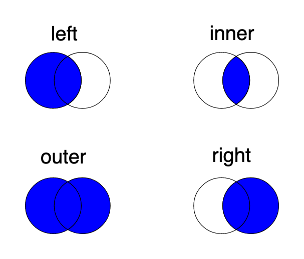
We could certainly clean the data by correcting some of the typos. Since the number of the rows with unknown states is not large (compared to the length of the whole dataset), we will deliberetly not fix the state names. Instead, we will remove those rows from the merged dataset by using the inner type of merge. All the merge types: left, inner, outer and right are well explained by the schema below:
We can use the merge function to add the "Population" values.
laser_incidents_w_population = pd.merge(
    laser_incidents, population, left_on="State", right_on="Territory", how="inner"
)laser_incidents_w_populationlaser_incidents_w_population.describe(include="all")Grouping & aggregation
A common pattern in data analysis is grouping (or binning) data based on some property and getting some aggredate statistics.
Example: Group this workshop participants by nationality a get the cardinality (the size) of each group.
Possibly the simplest group and aggregation is the value_counts method, which groups by the respective column value
and yields the number (or normalized frequency) of each unique value in the data.
laser_incidents_w_population["State"].value_counts(normalize=False)State
California 7268
Texas 3620
Florida 2702
Arizona 1910
Colorado 988
Washington 982
Kentucky 952
Illinois 946
New York 921
Puerto Rico 912
Oregon 895
Tennessee 888
Nevada 837
Pennsylvania 826
Indiana 812
Utah 789
Ohio 750
Georgia 714
North Carolina 605
Missouri 547
Minnesota 531
New Jersey 519
Michigan 505
Hawaii 500
Alabama 473
Virginia 412
Oklahoma 412
New Mexico 401
Louisiana 351
Massachusetts 346
South Carolina 306
Maryland 255
Idaho 237
Arkansas 237
Wisconsin 207
Iowa 200
Connecticut 185
District of Columbia 183
Kansas 172
Mississippi 156
Montana 134
Nebraska 112
West Virginia 108
North Dakota 92
New Hampshire 86
Rhode Island 81
Alaska 67
Maine 66
South Dakota 52
Delaware 43
Guam 31
Vermont 28
Wyoming 22
U.S. Virgin Islands 1
Name: count, dtype: int64This is just a primitive grouping and aggregation operation, we will look into more advanced patterns.
Let us say we would like to get some numbers (statistics) for individual states.
We can groupby the dataset by the "State" column:
grouped_by_state = laser_incidents_w_population.groupby("State")What did we get?
grouped_by_state<pandas.core.groupby.generic.DataFrameGroupBy object at 0x127bf6f60>What is this DataFrameGroupBy object? Its use case is:
Splitting the data into groups based on some criteria.
Applying a function to each group independently.
Combining the results into a data structure.
Let’s try a simple aggregate: the mean of altitude for each state:
grouped_by_state["Altitude"].mean().sort_values()State
Puerto Rico 3552.996703
Hawaii 4564.536585
Florida 4970.406773
Alaska 5209.848485
Wisconsin 5529.951220
New York 5530.208743
Guam 5800.000000
Maryland 6071.739130
District of Columbia 6087.144444
New Jersey 6204.306950
Illinois 6306.310566
Massachusetts 6473.763848
Texas 6487.493759
Delaware 6602.380952
Arizona 6678.333158
Nevada 6730.037485
California 6919.705613
Washington 7110.687629
Louisiana 7276.276353
Nebraska 7277.321429
Michigan 7330.459082
Oregon 7411.285231
South Dakota 7419.607843
North Dakota 7455.434783
Ohio 7482.409880
Pennsylvania 7518.614724
Connecticut 7519.562842
Vermont 7610.714286
Idaho 7636.756410
Oklahoma 7678.803440
Montana 7780.620155
Virginia 7903.889976
Rhode Island 8186.875000
Minnesota 8191.869811
South Carolina 8593.535948
Kansas 8661.994152
Indiana 8664.055693
Maine 8733.333333
Alabama 8821.210191
Mississippi 8828.685897
Tennessee 8987.354402
North Carolina 9251.180763
New Hampshire 9591.764706
Utah 9892.935197
Iowa 10174.619289
Missouri 10548.161468
New Mexico 10714.706030
U.S. Virgin Islands 11000.000000
Georgia 11130.663854
Arkansas 11203.483051
Colorado 11301.869388
Kentucky 11583.086225
West Virginia 12108.386792
Wyoming 18238.095238
Name: Altitude, dtype: float64What if we were to group by year? We don’t have a year column but we can just extract the year from the date and use it for groupby.
grouped_by_year = laser_incidents_w_population.groupby(laser_incidents_w_population["timestamp"].dt.year)You may have noticed how we extracted the year using the .dt accessor.
We will use .dt even more below.
Let’s calculate the mean altitude of laser incidents per year. Are the lasers getting more powerful? 🤔
mean_altitude_per_year = grouped_by_year["Altitude"].mean().sort_index()
mean_altitude_per_year
timestamp
2015.0 6564.621830
2016.0 7063.288912
2017.0 7420.971064
2018.0 7602.049323
2019.0 8242.586268
2020.0 8618.242465
Name: Altitude, dtype: float64We can also quickly plot the results, more on plotting in the next lessons.
mean_altitude_per_year.plot(kind="bar");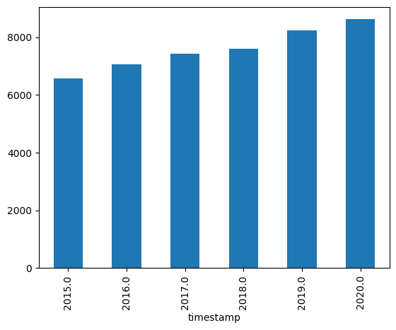
Exercise: Calculate the sum of injuries per year. Use the fact that True + True = 2 ;)
We can also create a new Series if the corresponding column does not exist in the dataframe and group it by another Series
(which in this case is a column from the dataframe). Important is that the grouped and the by series have the same index.
# how many incidents per million inhabitants are there for each state?
incidents_per_million = (1_000_000 / laser_incidents_w_population["Population"]).groupby(laser_incidents_w_population["State"]).sum()
incidents_per_million.sort_values(ascending=False)
State
Hawaii 347.174968
Puerto Rico 283.072541
District of Columbia 272.401284
Nevada 263.392087
Arizona 259.539186
Utah 233.376716
Oregon 211.078085
Kentucky 210.978412
New Mexico 189.746676
California 186.218871
Colorado 169.180226
Washington 126.127279
Tennessee 125.933528
Idaho 122.225872
Florida 121.466464
Texas 120.547839
Montana 119.337375
Indiana 118.834422
North Dakota 118.060573
Oklahoma 102.492661
Alabama 93.214901
Minnesota 92.877892
Alaska 91.332542
Missouri 88.540597
Arkansas 77.816234
Louisiana 76.466573
Illinois 75.186584
Rhode Island 74.058226
Georgia 65.427299
Ohio 63.796895
Pennsylvania 63.675570
Iowa 62.489904
New Hampshire 61.638539
West Virginia 60.839723
Kansas 58.560169
South Carolina 57.925648
South Dakota 57.153911
Nebraska 56.912796
North Carolina 56.547484
New Jersey 56.037235
Mississippi 53.060196
Connecticut 51.017524
Michigan 50.328315
Massachusetts 49.556186
Maine 47.641734
Virginia 47.445656
New York 46.805556
Vermont 43.272381
Delaware 42.223261
Maryland 41.364812
Wyoming 37.840934
Wisconsin 35.129169
U.S. Virgin Islands 0.000000
Guam 0.000000
Name: Population, dtype: float64incidents_per_million.sort_values(ascending=False).plot(kind="bar", figsize=(15, 3));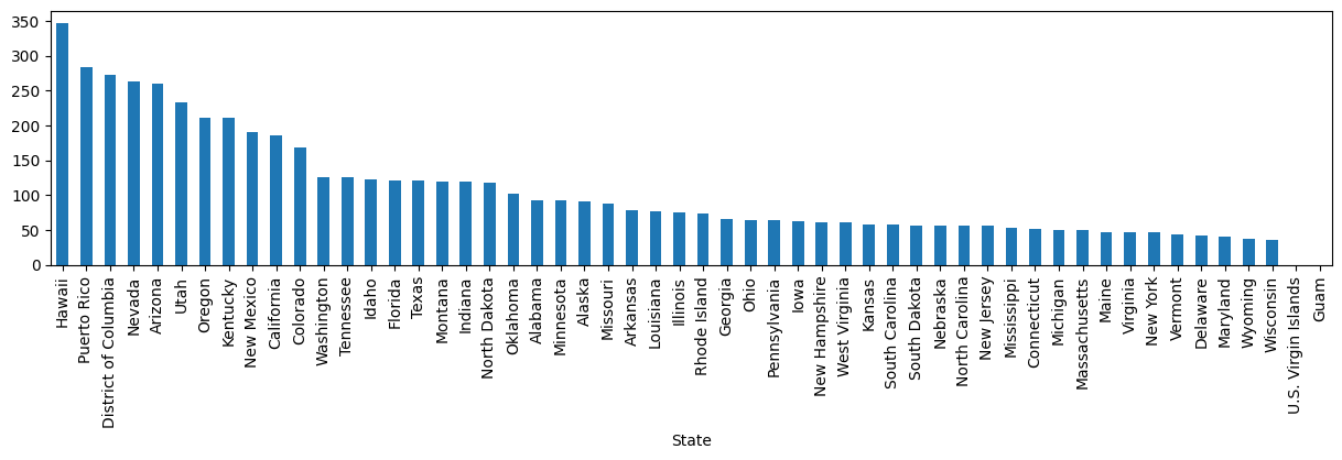
Time series operations (Optional)
We will briefly look at some more specific operation for time series data (data with a natural time axis). Typical operations for time series are resampling or rolling window transformations such as filtering. Note that Pandas is not a general digital signal processing library - there are other (more capable) tools for this purpose.
First, we set the index to "timestamp" to make our dataframe inherently time indexed. This will make doing further time operations easier.
incidents_w_time_index = laser_incidents.set_index("timestamp")
incidents_w_time_indexFirst, turn the data into a time series of incidents per hour. This can be done by resampling to 1 hour and using
count (basically on any column or on any column that has any non-NA value) to count the number of incidents.
incidents_hourly = incidents_w_time_index.notna().any(axis="columns").resample("1H").count().rename("incidents per hour")
incidents_hourly
/var/folders/dm/gbbql3p121z0tr22r2z98vy00000gn/T/ipykernel_95281/3245646514.py:1: FutureWarning: 'H' is deprecated and will be removed in a future version, please use 'h' instead.
incidents_hourly = incidents_w_time_index.notna().any(axis="columns").resample("1H").count().rename("incidents per hour")
timestamp
2015-01-01 02:00:00    1
2015-01-01 03:00:00    2
2015-01-01 04:00:00    1
2015-01-01 05:00:00    3
2015-01-01 06:00:00    0
                      ..
2020-08-01 06:00:00    0
2020-08-01 07:00:00    1
2020-08-01 08:00:00    1
2020-08-01 09:00:00    0
2020-08-01 10:00:00    3
Name: incidents per hour, Length: 48945, dtype: int64
Looking at those data gives us a bit too detailed information.
incidents_hourly.sort_index().plot(kind="line", figsize=(15, 3));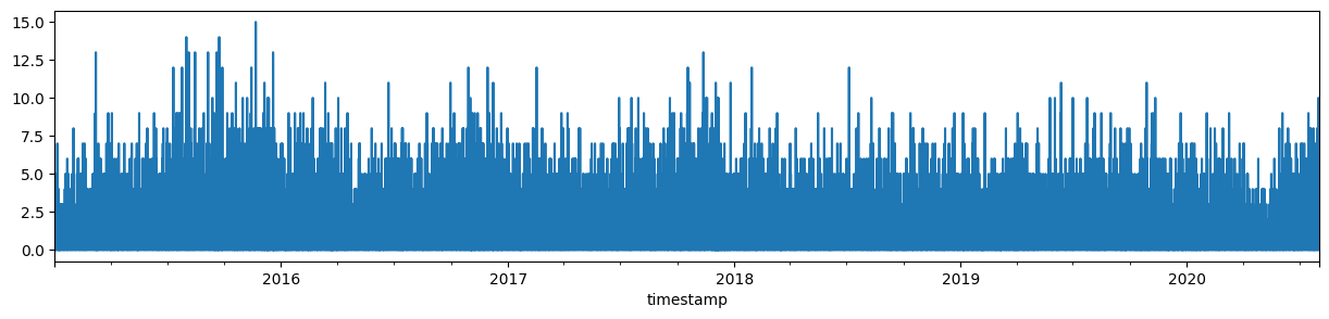
A daily mean, the result of resampling to 1 day periods and calculating the mean, is already something more digestible. Though still a bit noisy.
incidents_daily = incidents_hourly.resample("1D").mean()
incidents_daily.plot.line(figsize=(15, 3));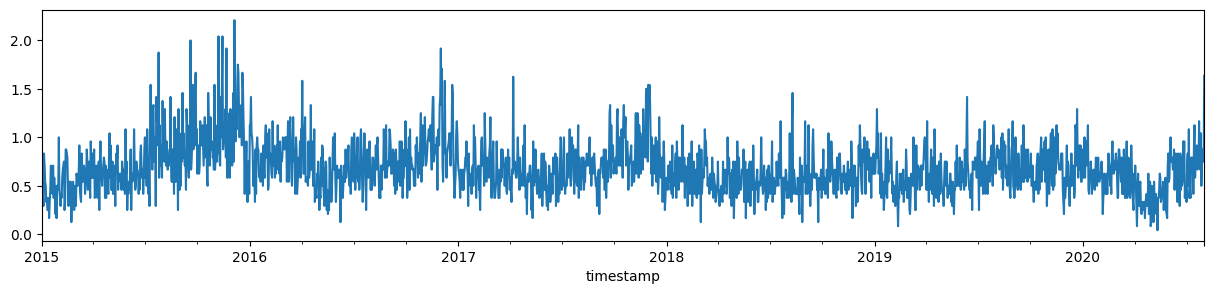
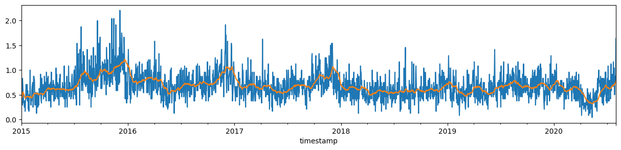
We can look at filtered data by rolling mean with, e.g., 28 days window size.
incidents_daily_filtered = incidents_daily.rolling("28D").mean()
incidents_daily.plot.line(figsize=(15, 3));
incidents_daily_filtered.plot.line(figsize=(15, 3));